Tuesday, February 8, 2011

Sorting Algorithms

Selection Sort
Selection sort is one of the O(n2) sorting algorithms where the minimal value is put in the start of the array. This sorting algorithm is inefficient on large lists, and generally performs worse than the similar insertion sort due to its computational complexity.

In selection sort, the array of inputs is imaginatively divided into two parts, the sorted and unsorted part. At the beginning, the sorted part is empty and the unsorted part is the whole array. In every loop, the algorithm looks for the smallest number from the unsorted array and then would swap it to the first element of the unsorted part. The loop stops until the unsorted part is empty.

Example. {10 14 73 25 23 13 27 94 33 39 25 59 94 65 82 45}


The C++ codes for the selection sort are the following:
void selectionSort(int arr[], int n) {
      int i, j, minIndex, tmp;    
      for (i = 0; i < n - 1; i++) {
            minIndex = i;
            for (j = i + 1; j < n; j++)
                  if (arr[j] < arr[minIndex])
                        minIndex = j;
            if (minIndex != i) {
                  tmp = arr[i];
                  arr[i] = arr[minIndex];
                  arr[minIndex] = tmp;
            }
      }
}


###########

Insertion Sort
Insertion sort is a simple sorting algorithm in which, just like the selection sort, belongs to the O(n2) sorting algorithms. It is a comparison sort in which the sorted array is built one entry at a time.It is much less efficient on large lists than more advanced algorithms such as quicksort, heapsort, or merge sort. However, it has a simple implementation and is efficient for small data sets.

Insertion sort works like selection sort. The array is also divided imaginatively into two parts. The sorted part is the array containing the first element and the unsorted part contains the rest of the inputs. In every loop, the algorithm inserts the first element from the unsorted part to its right position in the sorted part. And the loop ends when the unsorted part is empty.

Example. {10 14 73 25 23 13 27 94 33 39 25 59 94 65 82 45}


The C++ codes for the insertion sort are the following:
void insertionSort(int arr[], int length) {
      int i, j, tmp;
      for (i = 1; i < length; i++) {
            j = i;
            while (j > 0 && arr[j - 1] > arr[j]) {
                  tmp = arr[j];
                  arr[j] = arr[j - 1];
                  arr[j - 1] = tmp;
                  j--;
            }
      }
}

###########

Bubble Sort
Bubble sort is a simple and well-known sorting algorithm. Bubble sort belongs to O(n2) sorting algorithms, which makes it quite inefficient for sorting large data volumes. Bubble sort is stable and adaptive.

Bubble sort works by comparing pair of adjacent elements from the beginning of an array and tests them if they are in reversed order. If the current element is greater than the next element, then the algorithm swaps them. The algorithm stops when there are no more elements to be swapped.

Example. {2 3 4 5 1}


The C++ codes for the insertion sort are the following:
void bubbleSort(int arr[], int n) {
      bool swapped = true;
      int j = 0;
      int tmp;
      while (swapped) {
            swapped = false;
            j++;
            for (int i = 0; i < n - j; i++) {
                  if (arr[i] > arr[i + 1]) {
                        tmp = arr[i];
                        arr[i] = arr[i + 1];
                        arr[i + 1] = tmp;
                        swapped = true;
                  }
            }
      }
}

###########

Shell Sort
Shell Sort is one of the oldest sorting algorithms which is named from Donald Shell in 1959. It is fast, easy to understand and easy to implement. However, its complexity analysis is a little more sophisticated. Shell sort is the generalization of the insertion sort which exploits the fact that insertion sort works efficiently on input that is already almost sorted.

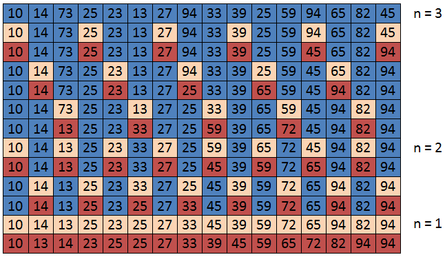
Shell sort algorithm does not actually sort the data itself but it increases the efficiency of other sorting algorithms, normally is the insertion sort. It works by quickly arranging data by sorting every nth element, where n can be any number less than half the number of data. Once the initial sort is performed, n is reduced, and the data is sorted again until n equals 1.

Choosing n is not as difficult as it might seem. The only sequence you have to avoid is one constructed with the powers of 2. Do not choose (for example) 16 as your first n, and then keep dividing by 2 until you reach 1. It has been mathematically proven that using only numbers from the power series {1, 2, 4, 8, 16, 32, ...} produces the worst sorting times. The fastest times are (on average) obtained by choosing an initial n somewhere close to the maximum allowed and continually dividing by 2.2 until you reach 1 or less. Remember to always sort the data with n = 1 as the last step.

Example. {10 14 73 25 23 13 27 94 33 39 25 59 94 65 82 45}


The C++ codes for the insertion sort are the following:
void shellsort (int[] arr, int length, int n) {
    int i, j, k, h, v;
    for (k=0; k < length; k++) {
        h=arr[k];
        for (i=h; i<n; i++) {
            v=arr[i];
            j=i;
            while (j>=h && arr[j-h]>v) {
                arr[j]=arr[j-h];
                j=j-h;
            }
            arr[j]=v;
        }
    }
}


Source:

Tuesday, February 1, 2011

Principles of Algorithm Analysis

Empirical Analysis deals with the analysis and characterization of the behavior of algorithms. It compares the performance of two algorithms by actually running them; meaning it is an analysis based on observations on executing them and not by getting results theoretically. With that, it requires a correct and complete implementation of the algorithm to be used.

Empirical analysis or empirical testing is useful because it may uncover unexpected interactions that affect performance, as it uses benchmarking which assess the relative performance of each algorithm every time it is implemented. With the continuous assessment of the algorithm, it could be optimized thoroughly and much more improvements could be made.

###########

Analysis of Algorithm is how is to determine the amount of resources (such as time and storage) necessary to execute a program. It provides theoretical estimates for the resources needed by any algorithm which solves a given computational problem. These estimates provide an insight into reasonable directions of search for efficient algorithms. In other words, it helps us know what and how much resources we need to efficiently solve a problem and to do it at low cost.

It may not be always possible to perform empirical analysis. Thus, we can resort to the analysis of algorithm, which is basically a mathematical analysis. Mathematical analysis may be theoretical that in such a way it could not actually solve the problem, but the point is that it is the most accurate way of analyzing an algorithm theoretically.

Mathematical analysis is actually more informative and less expensive but it can be difficult if we do not know all the mathematical formulas needed to analyze an algorithm. Thus, to do this process, one must have any skills in mathematics even it is just enough to be able to do the proper analysis of algorithms.

###########

Big-Oh Notation describes the behavior of a function for big inputs. It tries to capture the core of a function. It also describes the limiting behavior of a function when the argument tends towards a particular value or infinity, usually in terms of simpler functions. By mathematical representation, it is defined as f(n) = O(g(n)) which is read as "f of n is big oh of g of n". To understand easier, let's have examples on different common orders of growth of big-oh.

O(1) or O of a Constant:  
bool IsFirstElementNull(String[] strings){
       if(strings[0] == null)
            return true;
       return false;
}
O(1) describes an algorithm that will always execute in the same time (or space) regardless of the size of the input data set.


O(N):
bool ContainsValue(String[] strings, String value){
       for(int i = 0; i < strings.Length; i++)
            if(strings[i] == value)
                  return true;
      return false;
}
O(N) describes an algorithm whose performance will grow linearly and in direct proportion to the size of the input data set. 

O(N2):
bool ContainsDuplicates(String[] strings){
      for(int i = 0; i < strings.Length; i++){
            for(int j = 0; j < strings.Length; j++){
                  if(i == j) // Don't compare with self
                        continue;
                  if(strings[i] == strings[j])
                        return true;
            }
      }
      return false;
}
O(N2) represents an algorithm whose performance is directly proportional to the square of the size of the input data set. This is common with algorithms that involve nested iterations over the data set. Deeper nested iterations will result in O(N3), O(N4) etc. 

O(2N):
O(2N) denotes an algorithm whose growth will double with each additional element in the input data set. The execution time of an O(2N) function will quickly become very large.

O(log N) or Logarithms:
Binary search is a technique used to search sorted data sets. It works by selecting the middle element of the data set, essentially the median, and compares it against a target value. If the values match it will return success. If the target value is higher than the value of the probe element it will take the upper half of the data set and perform the same operation against it. Likewise, if the target value is lower than the value of the probe element it will perform the operation against the lower half. It will continue to halve the data set with each iteration until the value has been found or until it can no longer split the data set.

This type of algorithm is described as O(log N). The iterative halving of data sets described in the binary search example produces a growth curve that peaks at the beginning and slowly flattens out as the size of the data sets increase e.g. an input data set containing 10 items takes one second to complete, a data set containing 100 items takes two seconds, and a data set containing 1000 items will take three seconds. Doubling the size of the input data set has little effect on its growth as after a single iteration of the algorithm the data set will be halved and therefore on a par with an input data set half the size. This makes algorithms like binary search extremely efficient when dealing with large data sets.


Source:
http://en.wikipedia.org/wiki/Empirical_algorithmics
http://en.wikipedia.org/wiki/Algorithm
http://www.cs.umsl.edu/~sanjiv/cs278/lectures/analysis.pdf 
http://en.wikipedia.org/wiki/Analysis_of_algorithms 
http://www.c2.com/cgi/wiki?BigOh 
http://xw2k.nist.gov/dads/HTML/bigOnotation.html 
http://en.wikipedia.org/wiki/Big_O_notation 
http://rob-bell.net/2009/06/a-beginners-guide-to-big-o-notation/